Table of Contents
Overview
Checking the news is limited to what location you are in and usually what the top stories of the day are for the source you enjoy looking at. What if news could be viewed in a different way? I thought it would be an interesting change if you could find news stories by looking at the overall sentiment in an area. Color gradients for sentiment could be shown for cities all around the globe so a user could select an area that looks highly positive or negative and see what top news stories might be causing this. I accomplished this using the very detailed database called GDELT.
GDELT, or the Global Database of Events, Language, and Tone, is a conglomeration of news stories and events dating back to 1979. GDELT summarizes over 300 categories, 60 attributes and thousands of emotions for millions of different themes. There are so many different aspects of this dataset that I can’t explain them all. If you are interested, check out the source information at here.
The portion of the dataset that I focused on is called the GKG, or Global Knowledge Graph. GKG reads the emotions from every news report using some of the most sophisticated named entity and geocoding algorithms in existance. I am using this emotion data to sum sentiments of news stories by cities to overlay on an interactive map web app. This post will go through the pipeline I used to feed the data from the GDELT dataset into a postgGIS database. Part two will show how I took the data from the database with django and created an interactive web app.
Bootstrapping
There are countless choices when putting together a data pipeline since there are so many different tools you can use. Initially I was going to use lambda triggers in AWS to export the data I needed into a postgres database for further querying. I decided this might not be robust enough for anything I decide to do with the data down the line.
Taking a slightly Agile approach, I wanted to just get an MVP app out so I started focusing on just getting the sentiment points onto an interactive map. Once that was done I could further add to the pipeline and start extracting any other data I needed from the vast GDELT database.
The main tool I used for the project was Airflow. It let me easily create a skeleton pipeline first and then later on I can add what I need with little changes. Since I was most likely going to do further computations other than adding sentiment, I wanted the project to be scalable. I decided to use AWS EMR clusters to run spark jobs for any transformations I needed. Although, I didn’t want these EMR clusters to run all the time so I automated launching and terminating instances when computation was required.

I found a pretty useful tool that AWS has called Cloudformation. Cloudformation is basically just a yaml file that you can define all of the resources you want to use and AWS will spin them up in the correct order of dependencies. There are many templates floating around so I found one that started an EC2 instance and an RDS database. If you want an example of how the yaml files are formatted, check out my github here.
Extraction
The GDELT database has two sources. One is the historical data that goes all the way back to 1979. This database has more than a terabyte of data. In the future I may apply some predictive modeling to my app but for now I will focus on the second source of data.
The second source is updated every 15 minutes in the form of file links on a webpage. There are three links on the updates page; GKG, events, and mentions. I am only concerned with the GKG file for now as it contains the sentiment data that I am going to use in my initial web app. In order to get these files, I set up my first DAG in airflow. This is less of a DAG and more of just a scheduled script, there is no real dependencies, the script just runs and then the second operator prints out a confirmed message.
The Airflow scheduler works in cron format and I have it set to run every fifteen minutes. Since I may do something with the other files later on, I wanted to be able to extract those as well. I created an S3 uploader class that makes use of the boto3 CLI for easy extraction to S3. The uploader methods basically just point to a target of the three files then download them locally, unzip the file, upload it to S3, and then delete the local file.

The file extraction is fairly simple. I also have the buckets I am extracting to delete the files after a day, that way I can just continuously aggregate whatever files are in the bucket at a time.
s3_upload_confirm = BashOperator(task_id='s3_upload_confirm',
                                 bash_command="echo 'New files uploaded to S3 raw buckets'",
                                 dag=dag)

upload_raw_files = BashOperator(task_id='upload_raw_files',
                                bash_command='python /root/airflow/dags/extract/raw_file_collection.py',
                                dag=dag)

upload_raw_files >> s3_upload_confirm
The acutual DAG is basically just running a bash script that extracts the files. Not much of a graph but it allows me to add to it later in case I wanted to do more than just put the files in S3.
Transformation
Working with Livy
Transformation was where I made good use of DAG functionality. EMR clusters can get expensive if they are run all the time and I only have so many credits left on my account. This is where serverless computing would have come in handy with Lambda but I was already set on Airflow.
To keep things clean in the DAG file, I created a library of functions that I would need from the boto3 Software Development Kit (SDK) in order to work with the clusters before I could make any transformations. This involved getting some metadata first about the EC2 instance being run from as well as security groups for the master and slaves of the cluster.

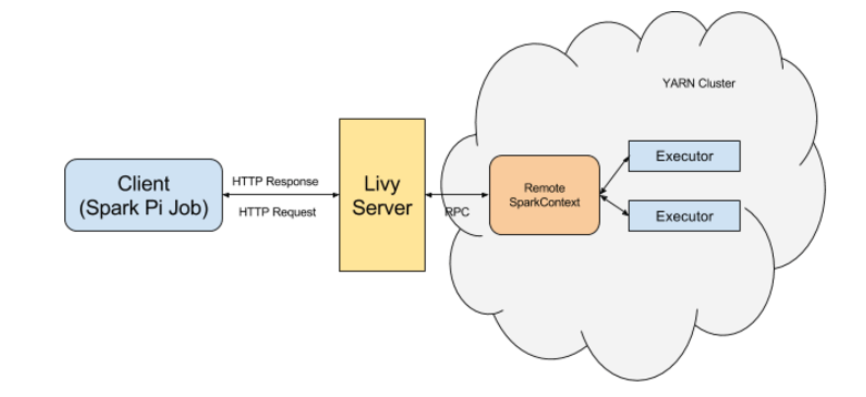
Instead of having to SSH into the cluster or set up step functions, I used the very useful REST interface called Apache Livy to submit spark jobs. All I have to do is submit a post request to the DNS of the cluster that has been created with according information for the headers and data of the session I create. Livy works over port 8998 and once I submit the request it will return a header with the information I can use for further querying.
def create_spark_session(master_dns, kind='spark'):
    # Livy server runs on port 8998 for interactive session
    host = 'http://' + master_dns + ':8998'
    data = {'kind': kind}
    headers = {'Content-Type': 'application/json'}
    response = requests.post(host + '/sessions', data=json.dumps(data), headers=headers)
    logging.info(response.json())
    return response.headers
Submitting a statement works in a similar way, however the url will include a /statements path and the data will be a json file containing the code that I need to execute to transform the data. In this case it is a scala script that I wrote.
Once the data is extracted, I can kill the cluster and wait a certain amount of time for files to build up in S3 again so the process can restart. The actual workflow looks like the below snippet.
create_cluster = PythonOperator(
    task_id='create_cluster',
    python_callable=create_emr,
    dag=dag)

wait_for_cluster_completion = PythonOperator(
    task_id='wait_for_cluster_completion',
    python_callable=wait_for_completion,
    dag=dag)

transform_geocam = PythonOperator(
    task_id='transform_geocam',
    python_callable=transform_geocam_sum,
    dag=dag)

terminate_cluster = PythonOperator(
    task_id='terminate_cluster',
    python_callable=terminate_emr,
    trigger_rule='all_done',
    dag=dag)

# construct the DAG by setting the dependencies
create_cluster >> wait_for_cluster_completion
wait_for_cluster_completion >> transform_geocam >> terminate_cluster
Data Transformation
Within the transform geocam DAG lies the actual scala code that does the transformation. The first thing I need to take care of for extraction is understanding the file format. The GKG files that are updated every 15 minutes are not very long files, only about two thousand rows. However, the files are very wide and end up each being around 15 MB. Depending on how long I make the cluster run, the build up could be fairly large.
The file has a total of 27 columns, each one containing some type of delimited values. So this dataset is essentially a relational flattened database. My focus is on column 18, this is where the GKG information lies and the column is called V2GCAM.
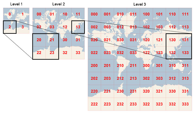
I mostly made use of spark-sql for the extraction in my scala file. To make summing the sentiments for cities easier, I used a geohashing function. Geohashing basically breaks the globe up into sections and the longer the hash, the more accurate the location. A twelve digit geohash is roughly a couple meters in accuracy. This makes it much easier to group by locations since I don’t have to worry about latitude and longitude.

The GCAM column that I need is comma delimited, so first I split the column up and then use the explode function to get all the different themes as their own row. There are a ton of themes that the GKG file records, so this makes the file considerably longer. However now if I want to query based on a certain theme, I can do so easily.
Once I create a user-defined function to geohash the locations, I can group the dataset by theme, geohash, date, and location for outputting back into S3. Then, my final DAG will take the file out of S3 and import it into a PostGIS database that will be queried by my django app.
