What makes a wine high quality has always been a mystery to me. Staring at the wine shelf can be daunting and I usually find myself picking the one with the nicest label. It just goes to show how important marketing is to the average person. So what exactly makes these wines high quality. Sometimes I can’t tell the difference between a $12 bottle and a $30 bottle. I decided to delve into the chemical makeup of wines to gain an understanding since all I knew before this was that wines can have legs.
The dataset of characteristics of red wine I used can be found here
This data set contained 1,599 variants of a Portuguese “Vinho Verde” wine. The main focus in this data set was the quality of the wine with 0 being poor and 10 being great quality. In order to understand how each feature effects quality, it was necessary to see how each feature is effected by each other. It was first necessary to understand what each of the qualities of wine were typically used for. Using a University of Californias lab study (http://waterhouse.ucdavis.edu/whats-in-wine) made it easier to obtain some domain knowledge and have a grasp of what each variable was.
A quick summary of the data will give an idea of the range of each variable:
summary(redwineinfo)
##        X          fixed.acidity   volatile.acidity  citric.acid
##  Min.   :   1.0   Min.   : 4.60   Min.   :0.1200   Min.   :0.000
##  1st Qu.: 400.5   1st Qu.: 7.10   1st Qu.:0.3900   1st Qu.:0.090
##  Median : 800.0   Median : 7.90   Median :0.5200   Median :0.260
##  Mean   : 800.0   Mean   : 8.32   Mean   :0.5278   Mean   :0.271
##  3rd Qu.:1199.5   3rd Qu.: 9.20   3rd Qu.:0.6400   3rd Qu.:0.420
##  Max.   :1599.0   Max.   :15.90   Max.   :1.5800   Max.   :1.000

##  residual.sugar     chlorides       free.sulfur.dioxide
##  Min.   : 0.900   Min.   :0.01200   Min.   : 1.00
##  1st Qu.: 1.900   1st Qu.:0.07000   1st Qu.: 7.00
##  Median : 2.200   Median :0.07900   Median :14.00
##  Mean   : 2.539   Mean   :0.08747   Mean   :15.87
##  3rd Qu.: 2.600   3rd Qu.:0.09000   3rd Qu.:21.00
##  Max.   :15.500   Max.   :0.61100   Max.   :72.00

##  total.sulfur.dioxide    density             pH          sulphates
##  Min.   :  6.00       Min.   :0.9901   Min.   :2.740   Min.   :0.3300
##  1st Qu.: 22.00       1st Qu.:0.9956   1st Qu.:3.210   1st Qu.:0.5500
##  Median : 38.00       Median :0.9968   Median :3.310   Median :0.6200
##  Mean   : 46.47       Mean   :0.9967   Mean   :3.311   Mean   :0.6581
##  3rd Qu.: 62.00       3rd Qu.:0.9978   3rd Qu.:3.400   3rd Qu.:0.7300
##  Max.   :289.00       Max.   :1.0037   Max.   :4.010   Max.   :2.0000

##     alcohol         quality
##  Min.   : 8.40   Min.   :3.000
##  1st Qu.: 9.50   1st Qu.:5.000
##  Median :10.20   Median :6.000
##  Mean   :10.42   Mean   :5.636
##  3rd Qu.:11.10   3rd Qu.:6.000
##  Max.   :14.90   Max.   :8.000
Univariate Plots Section
This data set contains information from 13 variables on 1,599 different types of wine. The quality of the wine is scored from 0 (worst) to 10 (best). However the actual values only range from 3 to 8.
ggplot(redwineinfo, aes(x = as.factor(quality))) +
  geom_histogram(stat = "count", color = 'black', fill = 'red') +
  scale_x_discrete(breaks = seq(0, 10))
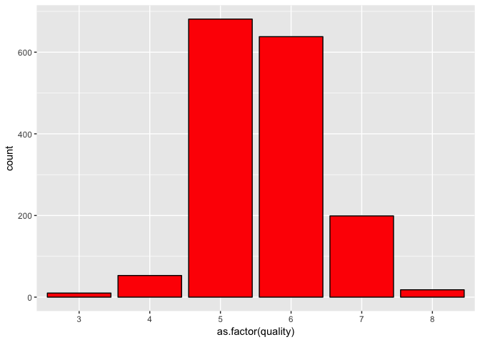
The bulk of wines in this data set are medium quality. There is a steep drop of quality before 5 and a slightly more gradual decrease in quality after 5. Separating these values in groups will make it easier to analyse what causes a wine to be a certain quality. The groups will be low, average, high.
redwineinfo$rating <-ifelse(redwineinfo$quality <= 4, 'Low',
                            ifelse(redwineinfo$quality <= 6, 'Average', 'High'))

redwineinfo$rating <- factor(redwineinfo$rating,
                             levels = c('Low','Average','High'))

ggplot(redwineinfo, aes(x = as.factor(rating))) +
  geom_histogram(stat = "count", color = 'black', fill = 'red')
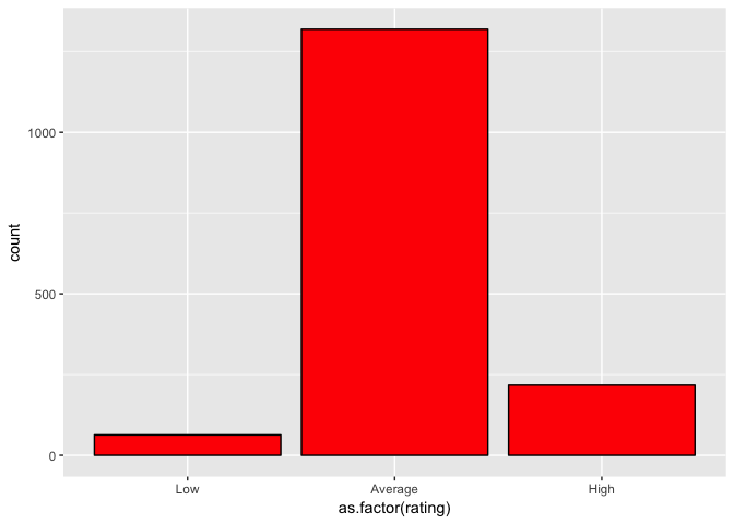
Separating the quality into categories shows a more clear distinction between high and low quality wines.
ggplot(redwineinfo, aes(x = alcohol)) +
  geom_histogram(binwidth = .1, color = 'black', fill = 'red3') +
  scale_x_continuous(breaks = seq(1, 20, .5))

summary(redwineinfo$alcohol)
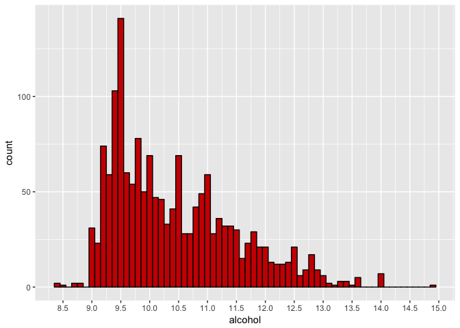
##    Min. 1st Qu.  Median    Mean 3rd Qu.    Max.
##    8.40    9.50   10.20   10.42   11.10   14.90
Observing each count of the variables shows different distributions and trends. In order to draw statistical conclusions with the data, it is most useful to transform the data to a normal distribution.
p1 <- ggplot(redwineinfo, aes(x = sulphates)) +
  geom_histogram(color = 'black', fill = 'orange')
p2 <- p1 + scale_x_log10()


grid.arrange(p1, p2, ncol = 2)
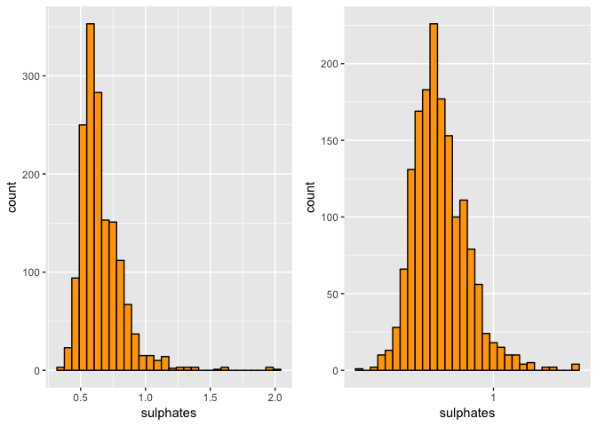
Sulphates has a slightly positively skewed distribution. Using a log10 transform shows a more normal distribution.
ggplot(redwineinfo, aes(x = pH)) +
  geom_histogram(binwidth = .05, color = 'black', fill = 'orange3') +
  scale_x_continuous(breaks = seq(2, 5, .1))

ggplot(redwineinfo, aes(x = density)) +
  geom_histogram(binwidth = .0005, color = 'black', fill = 'purple') +
  scale_x_continuous(breaks = seq(.9, 1.1, .001))
![image[center]](/assets/images/wineproject/unnamed-chunk-7-2.png)
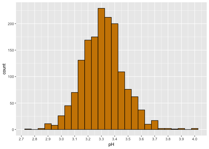
Density and pH have normal distributions, no transform is needed. Density is dependent on alcohol and sugar content so these variables will be compared later in the project
p1 <- ggplot(redwineinfo, aes(x = total.sulfur.dioxide)) +
  geom_histogram(color = 'black', fill = 'purple3')
p2 <- p1 + scale_x_log10()

p3 <- ggplot(redwineinfo, aes(x = free.sulfur.dioxide)) +
  geom_histogram(color = 'black', fill = 'yellow')
p4 <- p3 +scale_x_log10()

grid.arrange(p1, p2, p3, p4, ncol = 2)
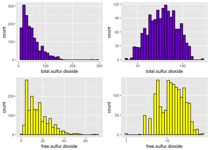
Total sulfur dioxide is dependent of free sulfur dioxide. Applying a log10 transform shows a normal distribution. However, free sulfur dioxide appears to be somewhat bimodal
p1 <- ggplot(redwineinfo, aes(x = chlorides)) +
  geom_histogram(color = 'black', fill = 'yellow3')
p2 <- p1 + scale_x_log10()

grid.arrange(p1, p2, ncol = 1)
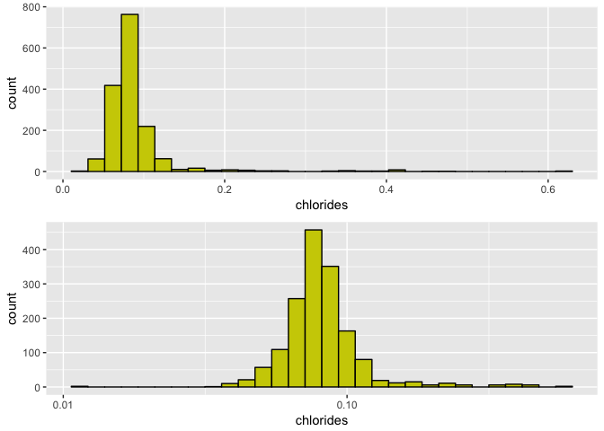
Chlorides has some outliers at .6 which is causing a positive skew. A log10 transform shows a more normal distribution
p1 <- ggplot(redwineinfo, aes(x = residual.sugar)) +
  geom_histogram(color = 'black', fill = 'blue')
p2 <- p1 + scale_x_log10()

p3 <- ggplot(redwineinfo, aes(x = citric.acid)) +
  geom_histogram(color = 'black', fill = 'blue3')
p4 <- p3 + scale_x_sqrt()

grid.arrange(p1, p2, p3, p4, ncol = 2)

ggplot(redwineinfo, aes(x = volatile.acidity)) +
  geom_histogram(binwidth = .05, color = 'black', fill = 'green') +
  scale_x_continuous(breaks = seq(.1, 1.6, .1))

ggplot(redwineinfo, aes(x = fixed.acidity)) +
  geom_histogram(binwidth = .5, color = 'black', fill = 'green3') +
  scale_x_continuous(breaks = seq(4, 16, 1))
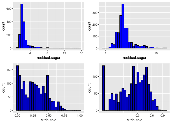
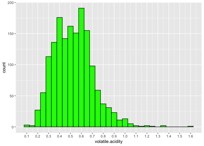
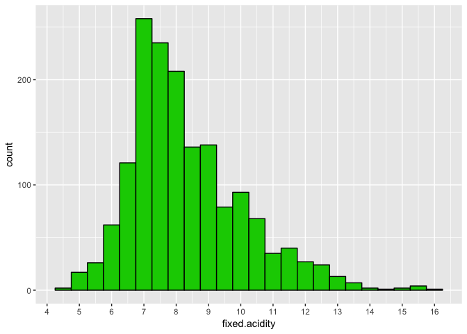
Citric acid has a decent amount of wines with an amount of 0. These values are still valid as wines are able to have no citric acid. Since this variable could have an effect on others, values of 0 will be kept in the data
Univariate Analysis
Dataset Structure
There are a total of 1,599 wines with 12 features for each wine. All features are numeric aside from Quality. The ordered variables for Quality are as follows
Quality: low (0-4) -> average(5-6) -> high(7-10)
Features of Interest
The main feature in this data set is quality. I want to see which features effect the quality of a wine in what ways. I suspect that pH and alcohol content will have a high effect. Through some research it looks like the “legs” of wine are caused by alcohol so it should have a high impact on quality. I created one variable that splits quality into categories for easier analysis on how each feature will effect it.
I used a log10 transform on any data that was positively skewed to obtain a more normal distribution. Citric acid has a decent amount of wines with the value of 0 so I used a square root transform for that feature. Many of these wines contain outliers but residual sugar and chlorides appear to be the most skewed. I wonder if these values are for the same type of wines and what cause a higher quality?
Bivariate Plots Section
# Test correlations
corTest <- function(x, y){
  return(cor.test(x, y)$estimate)
}

corList <- c(
  corTest(redwineinfo$fixed.acidity, redwineinfo$quality),
  corTest(redwineinfo$volatile.acidity, redwineinfo$quality),
  corTest(redwineinfo$citric.acid, redwineinfo$quality),
  corTest(redwineinfo$residual.sugar, redwineinfo$quality),
  corTest(redwineinfo$chlorides, redwineinfo$quality),
  corTest(redwineinfo$free.sulfur.dioxide, redwineinfo$quality),
  corTest(redwineinfo$total.sulfur.dioxide, redwineinfo$quality),
  corTest(redwineinfo$density, redwineinfo$quality),
  corTest(redwineinfo$pH, redwineinfo$quality),
  corTest(redwineinfo$sulphates, redwineinfo$quality),
  corTest(redwineinfo$alcohol, redwineinfo$quality)
)
names(corList) <- c('fixed acidity', 'volatile acidity', 'citric acid',
                    'residual sugar', 'chlorides', 'free sulfur dioxide',
                    'total sulfur dioxide', 'density', 'pH', 'sulphates',
                    'alcohol')
sort(corList)
##     volatile acidity total sulfur dioxide              density
##          -0.39055778          -0.18510029          -0.17491923
##            chlorides                   pH  free sulfur dioxide
##          -0.12890656          -0.05773139          -0.05065606
##       residual sugar        fixed acidity          citric acid
##           0.01373164           0.12405165           0.22637251
##            sulphates              alcohol
##           0.25139708           0.47616632
Observing each of the factors correlation to quality shows that no single attribute of wine has a clear effect on the quality. This could be due to a large quantity of wines being average. Making a high quality wine looks to be a mix of multiple different attributes with no dominating factor. Taking a closer look at the four highest correlated attributes could lead to some conclusions
theme_set(theme_minimal(10))
set.seed(1345)
wine_subset <- redwineinfo[c('volatile.acidity','citric.acid',
                             'sulphates','alcohol')]
wine_samp <- wine_subset[sample(1:length(wine_subset$alcohol), 1000), ]

ggpairs(data = wine_samp,
        lower = list(continuous = wrap("points", alpha=0.5, size=0.2),
                     discrete=wrap('box', size = 2)),
        upper = list(continuous = wrap("cor", size=3),
                     combo=wrap('box', size =0.3, outlier.size=0.2)),
        axisLabels = "show")
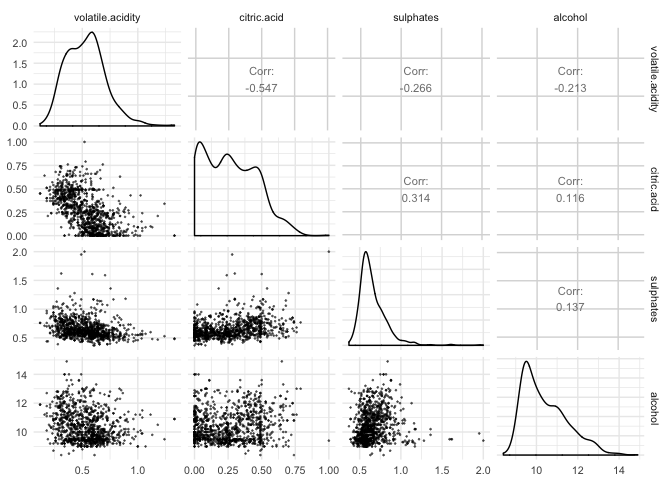
The stronget correlation so far appears to be between citric acid and volatile acidity. There also appears to be some correlation with sulphates and citric acid. Lets see how each of these variables effect the quality of wine separately
theme_set(theme_minimal(10))

plt1 <- ggplot(data = redwineinfo, aes(x=volatile.acidity, fill = rating)) +
  geom_histogram(position = position_stack(reverse = TRUE))
print(plt1)
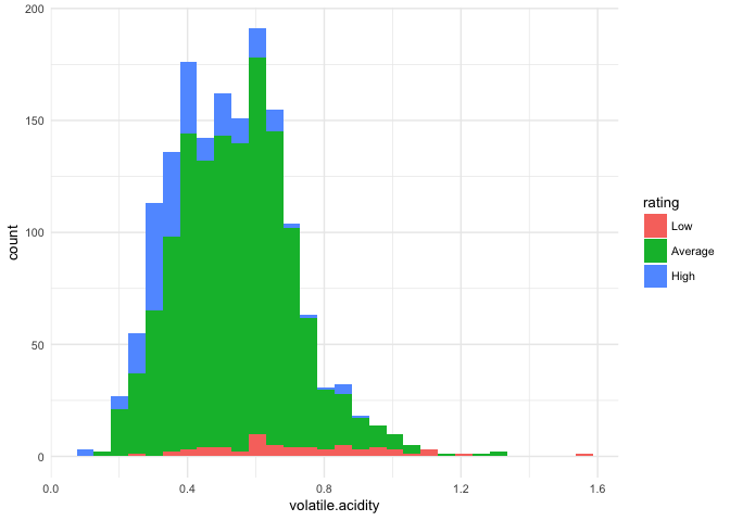
Observing the counts in each quality group for the wine, it is clear that high quality wines tend to have less volatile acidity. Wine spoilage is defined by the volatile acidity, which in large quantities gives the taste of vinegar. Low amounts are kept in high quality wines to keep a complex taste
plt1 <- ggplot(data = redwineinfo, aes(x=citric.acid, fill = rating)) +
  geom_histogram(binwidth = .02, position = position_stack(reverse = TRUE))
print(plt1)
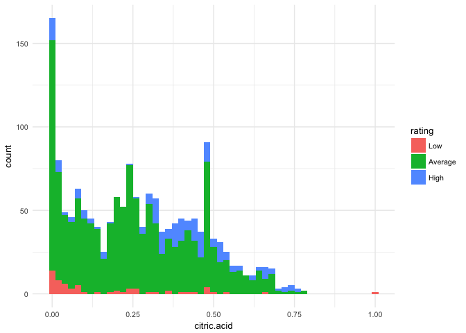
This is a somewhat mixed result. However the bulk of high quality wines have a higher amount of citric acid and lower quality has less, some even none. Citric acid could be a factor in high quality wine, although the largest outlier is also a low quality wine. Having no citric acid does not mean a wine cannot be high quality either
plt1 <- ggplot(data = redwineinfo, aes(x=sulphates, fill = rating)) +
  geom_histogram(binwidth = .02, position = position_stack(reverse = TRUE))
print(plt1)
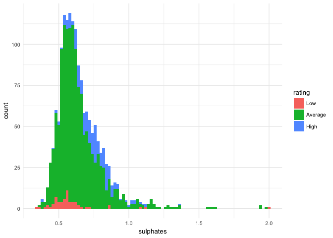
Overall it looks like having more sulphates could lead to higher quality wines. Once again there is also a low quality outlier. Sulphates are used as a preservative in wine and they are naturally produced by yeast during fermentation so all wines typically have them
plt1 <- ggplot(data = redwineinfo, aes(x=alcohol, fill = rating)) +
  geom_histogram(binwidth = .2, position = position_stack(reverse = TRUE))
print(plt1)
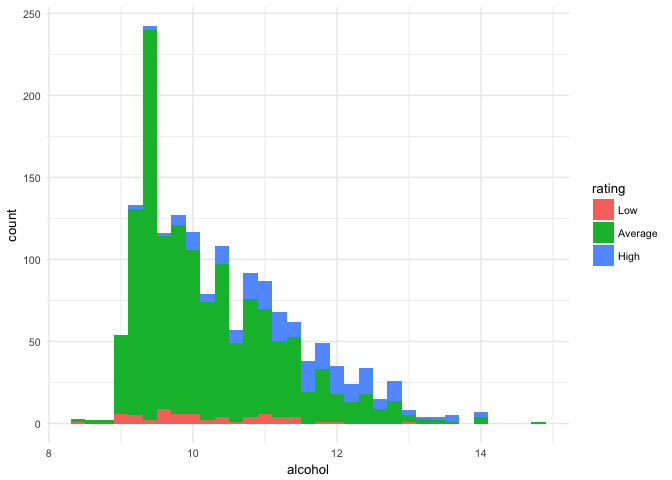
It is clear that a higher alcohol content is associated with higher quality wines. Although these wine attributes correlate with the main feature, quality, there may be stronger correlations between other attributes. From the correlation matrix above, it shows that citric acid and volatile acidity are negatively correlated (-.559), but what about fixed acidity?
ggplot(data = redwineinfo, aes(x=citric.acid, y=fixed.acidity)) +
  geom_point(alpha = .5) + geom_smooth(method = 'lm')

cor.test(redwineinfo$citric.acid, redwineinfo$fixed.acidity,
                    method = "pearson")
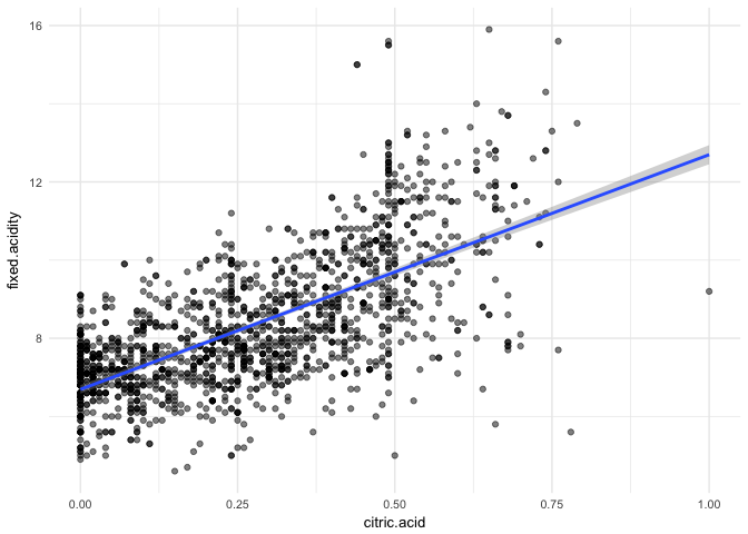
##
##  Pearson's product-moment correlation
##
## data:  redwineinfo$citric.acid and redwineinfo$fixed.acidity
## t = 36.234, df = 1597, p-value < 2.2e-16
## alternative hypothesis: true correlation is not equal to 0
## 95 percent confidence interval:
##  0.6438839 0.6977493
## sample estimates:
##       cor
## 0.6717034
This positive relationship would make sense when you understand what each variable is. Fixed acids in wine are acids that do not evaporate easily. The predominant fixed acids in wines are tartaric, malic, citric, and succic. So it would make sense that citric acid is positively correlated with tartaric acid (the specific acid that fixed acidity was measured from). Fixed acids in wine contribute a lot to the tase. However, correlation with quality is fairly low. This is due to high quality wines having a very specific amount of fixed acids. Too little and the wine will be flat, too much and the wine will taste sour.
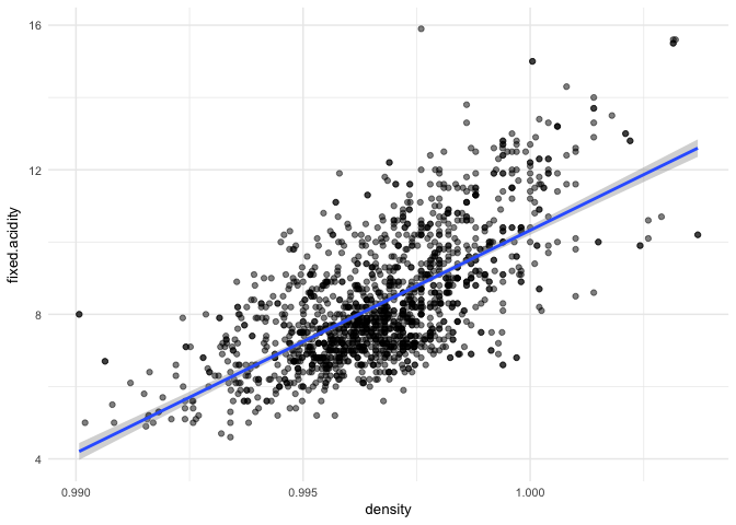
ggplot(data = redwineinfo, aes(x=density, y=fixed.acidity)) +
  geom_point(alpha = .5) +
  geom_smooth(method = 'lm')

cor.test(redwineinfo$density, redwineinfo$fixed.acidity,
                    method = "pearson")
##
##  Pearson's product-moment correlation
##
## data:  redwineinfo$density and redwineinfo$fixed.acidity
## t = 35.877, df = 1597, p-value < 2.2e-16
## alternative hypothesis: true correlation is not equal to 0
## 95 percent confidence interval:
##  0.6399847 0.6943302
## sample estimates:
##       cor
## 0.6680473
Knowing that fixed acidity is acids that do not evaporate readily, it would be expected that more dense wines have more fixed acids.
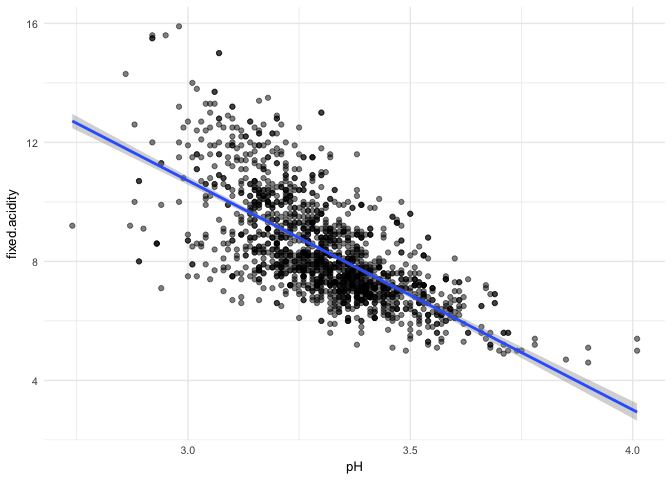
ggplot(data = redwineinfo, aes(x=pH, y=fixed.acidity)) +
  geom_point(alpha = .5) +
  geom_smooth(method = 'lm')

cor.test(redwineinfo$pH, redwineinfo$fixed.acidity,
                    method = "pearson")
##
##  Pearson's product-moment correlation
##
## data:  redwineinfo$pH and redwineinfo$fixed.acidity
## t = -37.366, df = 1597, p-value < 2.2e-16
## alternative hypothesis: true correlation is not equal to 0
## 95 percent confidence interval:
##  -0.7082857 -0.6559174
## sample estimates:
##        cor
## -0.6829782
pH describes how acidic a wine is from 0 (very acidic) to 14 (very basic). This plot follows that definition as the more acidic a wine becomes, the lower on the pH scale it is.
Bivariate Analysis
High quality wines appear to be associated with a specific amount of each chemical attribute. No single characteristic had a strong relationship with the feature of interest, quality. The characteristics with the greatest relation to quality were volatile acidity, citric acid, sulphates, and alcohol. Separating quality into low, average, and high resulted in a clear plot to see how each characteristic effects wine quality. High quality wines generally have less volatile acidity. Wine spoilage is defined by volatile acidity and is what gives a taste of vinegar. This is not to be confused with fixed acidity, which will have a wine taste flat with too little, and sour with too much. Fixed acidity has a large impact on taste, so why a low correlation with quality? That is due to high quality wines having a specific amount of fixed acidity, not too much or too little.
Correlations
There were stronger correlations between other variables than there were with quality. Fixed acidity is a measure of acids that do not evaporate easily. The main types that make up fixed acidity being tartaric, malic, citric, and succic. So there was an expected positive correlation between citric acid and fixed acidity (tartaric acid). Fixed acidity also had strong correlation with pH and density. If a wine has more acids that do not evaporate readily, it should make sense that they would be more dense. Lower pH numbers means the wine would have more acids present, so that correlation also makes sense
The strongest relationship was between fixed acidity and pH with an r2 value of -.68
Multivariate Plots Section
ggplot(data = redwineinfo, aes(x=as.factor(quality), y=alcohol)) +
  geom_jitter(aes(color=rating)) +
  geom_boxplot(outlier.shape = NA, alpha = .5) +
  labs(x="Quality Rating",                                                                                                    y="Alcohol (% by Volume)",                                                                                             color = "Quality Category",                                                                                            title = "Red Wine Quality and Alcohol Content")
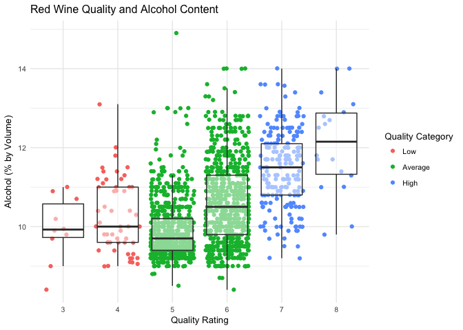
Alcohol content is the highest correlated to quality. This boxplot clearly shows that high quality wines typically have higher alcohol content
ggplot(data = redwineinfo, aes(x=citric.acid, y=fixed.acidity,
                               color = rating)) + geom_point() +
  geom_smooth(method = 'lm')
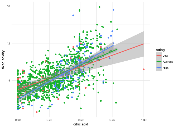
All quality wines are fairly close on the scale however it looks like high quality wines typically have more citric acid and tartaric acid
ggplot(data = redwineinfo, aes(x=density, y=fixed.acidity, color = rating)) +
  geom_point() + geom_smooth(method = 'lm')
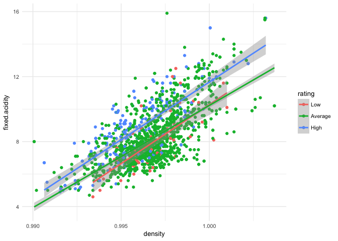
Average and low quality wines dont have a clear difference here. However, high quality wines have a clear separation being less dense with the same fixed acidity, and more fixed acids for the same density
ggplot(data = redwineinfo, aes(x=volatile.acidity, y=fixed.acidity,
                               color = rating)) + geom_point() +
  geom_smooth(method = 'lm')
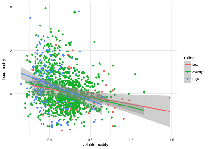
High quality wines usually have less volatile acidity. There is also on average more fixed acidity which follows the past plots
ggplot(data = redwineinfo, aes(x=pH, y=fixed.acidity, color = rating)) +
  geom_point() + geom_smooth(method = 'lm')
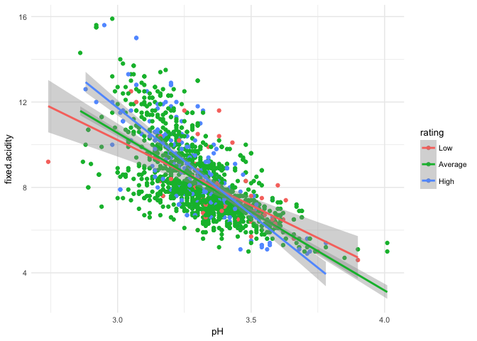
Once again, high quality wines have a higher fixed acidity. That would mean they are more acidic which is clear from this graph
ggplot(data = redwineinfo, aes(x=alcohol, y=fixed.acidity, color = rating)) +
  geom_point() + geom_smooth(method = 'lm')
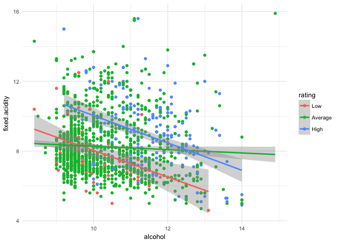
Fixed acidity and alcohol have had an impact on quality in past plots. Here it can clearly be seen that higher quantities of both relate to high quality wines.
Multivariate Analysis
Fixed acidity and citric acid when paired together were associated with higher quality wines. When citric acid was lower, wine quality was also lower. While fixed acidity is a measurement of multiple different acids, citric acid appears to have a stronger impact on quality than tartaric does. For low amounts of citric acid, tartaric acid might not have the same impact on quality that citric acid does.
Fixed acidity and alcohol content had an interesting relationship. There does not appear to be any correlation between the two, however there is a clear separation between high and low quality wines.
Final Plots and Summary
Plot One
ggplot(data = redwineinfo, aes(x=as.factor(quality), y=alcohol)) +
  geom_jitter(aes(color=rating)) +
  geom_boxplot(outlier.shape = NA, alpha = .5) +
  labs(x="Quality Rating",                                                                                                    y="Alcohol (% by Volume)",                                                                                             color = "Quality Category",                                                                                            title = "Red Wine Quality and Alcohol Content")
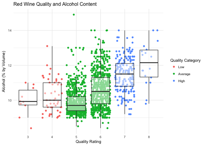
Description One
Many factors have to do with making a high quality wine. Out of all attributes, alcohol content had the strongest impact on whether a wine is high quality or not. With an r2 value of .476, it is the highest correlated factor to quality
Plot Two
ggplot(data = redwineinfo, aes(x=density, y=fixed.acidity, color = rating)) +
  geom_point() + geom_smooth(method = 'lm') +
  labs(x="Density (g/cm^3)",                                                                                                  y="Tartaric Acid (g/dm^3)",                                                                                            color = "Quality Category",                                                                                            title = "Red Wine Quality from Fixed Acidity vs. Density")
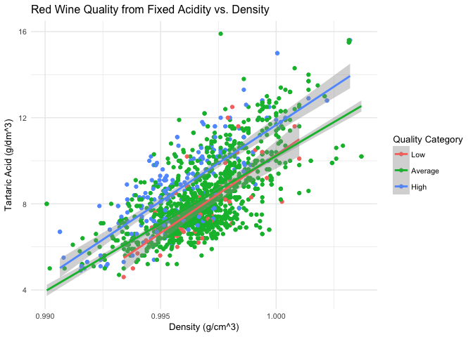
Description Two
Earlier plots showed that fixed acids could cause a wine to be more dense due to not evaporating readily. Looking at this plot, at the same acid content, high quality wines are noticably less dense than average or low quality wines. This would mean there is some characteristic that high quality wines could have that makes them less dense than other wines.
Plot Three
ggplot(data = redwineinfo, aes(x=alcohol, y=fixed.acidity, color = rating)) +
  geom_point() + geom_smooth(method = 'lm') +
  labs(x="Alcohol (% by Volume)",                                                                                             y="Tartaric Acid (g/dm^3)",                                                                                            color = "Quality Category",                                                                                            title = "Red Wine Quality from Fixed Acidity vs. Alcohol Content")
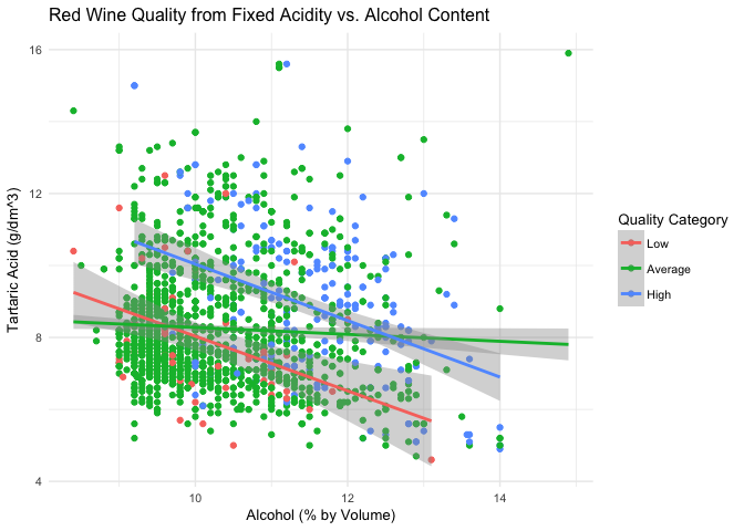
Description Three
Fixed acids are a main contributor to the taste of wines, and alcohol content has strong correlations related to quality. These two factors together give a clear separation to low and high quality wines. Even though there is no strong correlation between the two characteristics, they tell a lot about their effect on quality. High quality wines tend to have larger quantities of both characteristics.
Reflection
The features volatile acidity, citric acid, sulphates, and alcohol had the strongest correlation with quality. My main focus was with the fixed acids and alcohol. I decided not to focus on volatile acidity as it has more to do with spoilage. Fixed acidity appeared to be a more interesting attribute as it was more of an effect on the taste of wine. Alcohol content was also a focus since the correlation to quality was so high (.476). It is difficult to pinpoint what makes a high quality wine since it could be a very specific mix of different variables. Although, alcohol and fixed acidity showed a clear separation between high and low quality wines.
These conclusions may have been limited by the dataset. Overall, a bulk of the wines were average quality. Had there been more high and low quality wines, it could have given a more clear result. This was somewhat resolved when breaking up into categories for quality, although some results were still unlclear. Some further exploration would be to have price included in the wines. It would also be interesting to do the same analysis on white wine and determine the differences.
